Getting Started

Start out by installing the package. The simplest way to do this is pip install autotuning_methodology. Python 3.9 and up are supported.

Defining an experiment

To get started, all you need is an experiments file. This is a json file that describes the details of your comparison: which algorithms to use, which programs to tune on which devices, the graphs to output and so on. A simple example experiments file is as follows:

{
    "version": "0.1.2", // schema version
    "name": "Example", // experiment name
    "folder_id": "example", // folder ID to write to (must be unique)
    "kernels_path": "../cached_data_used/kernels", // path to the kernels
    "bruteforced_caches_path": "../cached_data_used/cachefiles", // path to the bruteforced cachefiles
    "visualization_caches_path": "../cached_data_used/visualizations", // path to the folder ID
    "kernels": [
        "convolution"
    ], // list of kernels to evaluate with
    "GPUs": [
        "RTX_3090"
    ], // list of GPUs to evaluate on
    "cutoff_percentile": 0.96, // percentile of distance between median and optimum at which to stop 
    "objective_time_keys": [ // list of keys to use as time objective
        "compilation",
        "benchmark",
        "framework",
        "search_algorithm",
        "validation"
    ],
    "objective_performance_keys": [ // list of keys to use as performance objective
        "time"
    ],
    "plot": {
        "plot_x_value_types": [
            "aggregated"
        ], // list of plot x-axis types
        "plot_y_value_types": [
            "baseline"
        ], // list of plot y-axis types
        "confidence_level": 0.95 // confidence level for the error shade
    },
    "strategy_defaults": { // these defaults are applied to all strategies
        "record_data": [
            "time",
            "GFLOP/s"
        ] // the data to record
        "stochastic": true, // whether the strategy has stochastic behaviour
        "iterations": 32, // number of times an individual configuration is repeated
        "repeats": 100, // number of times a strategy is repeated
        "minimum_number_of_evaluations": 20, // minimum number of non-error results to count as a single run
    },
    "strategies": [ // the list of strategies or algorithm to evaluate
        {
            "name": "genetic_algorithm", // the name of the strategy (for internal use, must be unique)
            "strategy": "genetic_algorithm", // the strategy as specified by the auto-tuning framework
            "display_name": "Genetic Algorithm" // the name of the strategy used in plots and other visualization
        },
        {
            "name": "ktt_profile_searcher",
            "strategy": "profile_searcher",
            "display_name": "KTT Profile Searcher"
        }
    ]
}

Running experiments

To use these experiment files, two entry points are defined: autotuning_experiment and autotuning_visualize. Both entrypoints take one argument: the path to the experiments file. The first runs the experiment and saves the results, the second visualizes the results. autotuning_experiment is intended for situations where you do not evaluate on the same machine as you visualize on (e.g. running on a cluster and visualizing on your laptop). If the results do not yet exists, autotuning_visualize will automatically trigger autotuning_experiment, so when running on the same machine, autotuning_visualize is all you need.

A note on file references

File references in experiments files are relative to the location of the experiment file itself. File references in tuning scripts are relative to the location of the tuning script itself. Tuning scripts need to have the global literals file_path_results and file_path_metadata for this package to know where to get the results. Plots outputted by this package are placed in a folder called generated_plots relative to the current working directory.

Processing Pipeline

To clarify the complex process of this package to obtain the results and visualize, the flowcharts below illustrate this pipeline.

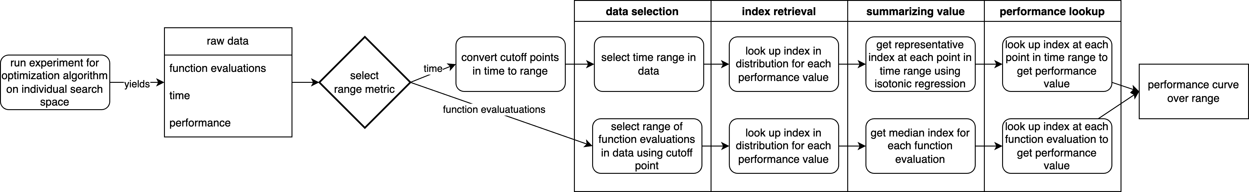
The first flowchart shows the tranformation of raw, stochastic optimization algorithm data to a performance curve.

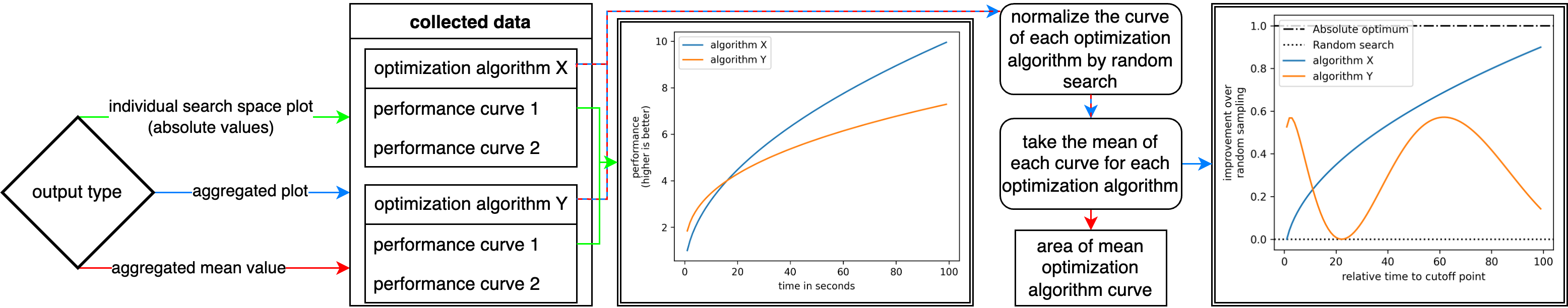
The second flowchart shows the adaption of performance curves of various optimization algorithms and search spaces to the desired output.